A Treasury security is a loan to the US government with defined repayment terms. The Treasury raises money to finance government operations and refinance maturing debt. At an auction, investors submit bids; the resulting price and yield establish the terms on which the government borrows. Afterwards, investors trade those securities with each other in the secondary market.

The primary and secondary markets perform different jobs. When Treasury issues a new security, it receives funding. When an investor later sells that security to another investor, the transaction normally changes its owner rather than providing fresh money to the government. Nevertheless, secondary-market prices influence the yield Treasury must offer at its next comparable auction. Existing debt and future financing are therefore connected through market prices.

An auction is a process for finding a clearing level, rather than an invitation for every investor to choose any desired return. Competitive bidders specify acceptable terms; non-competitive participants accept the result. Successful bids are allocated under the auction rules. A strong government borrower can still face a higher clearing yield if investors have better alternatives or are being asked to absorb more debt.

The main instruments differ by maturity and payment structure. Bills mature within a year and typically deliver their return through the difference between the purchase price and face value. Notes mature in two to ten years, while bonds have twenty- or thirty-year terms. Notes and bonds generally pay a fixed coupon every six months. TIPS adjust their principal with US consumer prices.

Banks, pension funds, insurers, foreign reserve managers and investment funds all participate. Their objectives differ: some need predictable income, others liquid collateral or protection during market stress. Treasuries also support repo transactions—short-term loans secured by securities—which helps explain why this market matters beyond government financing.

The benchmark role extends to private borrowing. A company raising long-term dollars often pays a Treasury-related base rate plus a credit spread, meaning extra compensation for lending to that company. If the Treasury benchmark rises while the spread stays unchanged, its potential borrowing cost increases. If the economy deteriorates, the spread can widen even when Treasury yields fall. Lower government borrowing costs need not mean easier funding for everyone.

“Safe” needs a precise meaning. Treasuries are a reference for low dollar credit risk, but their market prices can fall sharply before maturity. Inflation can erode purchasing power, and an investor measuring wealth in another currency also faces exchange-rate risk. A long-duration Treasury fund is therefore very different from cash.

Liquidity means that a security can generally be traded without an excessive price concession, but liquidity is not guaranteed at every moment. Dealers connect buyers and sellers while managing inventory and balance-sheet limits. During stress, the price needed to sell immediately may worsen. Investors should therefore distinguish the government’s ability to meet a payment from the trading conditions prevailing when they want to exit.

Consider a pension fund holding a ten-year note to meet a future obligation and a leveraged trader using the same note as collateral. A price decline affects both on paper, but the trader may face demands for additional collateral long before maturity. The pension fund’s objective and funding arrangements may allow more patience. Identical securities can generate very different decisions because the owners’ liabilities and financing differ.

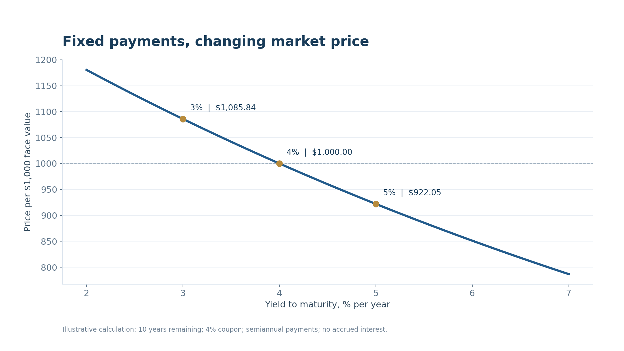
Imagine a newly issued ten-year note with a $1,000 face value and a 4% annual coupon. Its payments total $40 a year, usually split into two $20 instalments. The coupon rate stays fixed. The price paid by the next buyer does not: it changes as competing investments and economic expectations change.

If comparable new debt offers 5%, the old note’s $40 annual payment becomes less attractive. Its price must fall until the combination of coupons and repayment at maturity offers a competitive yield. With exactly ten years remaining and semiannual payments, its theoretical price at a 5% yield is about $922.05. At a 3% yield it is about $1,085.84. This example excludes accrued interest, fees and taxes.

The inverse relationship follows from the payments rather than from a market convention. The old note cannot raise its coupon to compete with a newly issued security. Its price is the variable that can adjust immediately. When investors accept a lower return, they can pay more for the same promised dollars. When they demand more, they must pay less. This logic applies before any view about the economy is added.

A one-year zero-coupon example makes the calculation even clearer. Pay $950 today and receive $1,000 in exactly one year: the holding-period return is $50 divided by $950, or approximately 5.26%, before costs. The return is not 5% of the amount invested, because the investor paid less than face value. Actual bill quotation conventions can differ, so quoted discount rates should not be compared mechanically with coupon-bond yields.

Current yield is annual coupon income divided by the purchase price. At $922.05 it is approximately 4.34%. Yield to maturity is different: it also incorporates the movement from the purchase price towards the $1,000 repayment. It is the discount rate that equates all promised payments to today’s price, rather than a promise about the investor’s realised annual return.

For a coupon bond, the calculation repeats this discounting for every payment. A dollar arriving six months from now is valued differently from a dollar arriving ten years from now. Yield to maturity combines all these payments into one annualised internal rate of return under the relevant convention. It is a convenient comparison tool, but it compresses the timing of cash flows into a single figure.

The price on a trading screen also needs context. Bond quotations may use a clean price excluding accrued coupon interest. The cash settlement amount normally includes the accrued amount because the seller has held the bond for part of the coupon period. That adjustment does not mean the buyer is receiving free extra income at the next coupon date. The worked chart deliberately uses a coupon-date valuation to isolate the price–yield mechanism.

Realised results depend on when the investor sells and on the rates available for reinvesting coupons. A holder who keeps the security to maturity receives its contractual payments, assuming payment as promised, but still bears inflation and opportunity costs. A bond fund normally maintains a portfolio rather than returning a fixed face value on the investor’s chosen exit date.

Suppose an investor buys the example at $922.05 and later sells after yields fall. The investor may earn a capital gain as well as coupon income, but the result depends on the remaining maturity and sale price. If yields rise instead, the near-term total return can be negative despite receiving interest. Income, price change and holding-period return should therefore be examined separately before being combined.

Illustrative price of a 4% coupon note with ten years remaining.View original ↗

The longer investors must wait for their money, the more sensitive its present value tends to be to a change in interest rates. Duration summarises that sensitivity. Modified duration of eight means that a small one-percentage-point rise in yield implies roughly an 8% price decline; a comparable fall implies roughly an 8% gain. This is an approximation, not a fixed rule.

Maturity and duration are related but not identical. Maturity is the date of the final principal payment. Duration also reflects the timing and size of the earlier coupons. A bond returning more money through early coupons generally has less sensitivity than a comparable bond whose payments arrive mostly at the end. A zero-coupon bond concentrates its entire payment at maturity and makes that timing effect especially visible.

A basis point is one hundredth of a percentage point. A move from 5.00% to 5.25% is therefore 25 basis points, not a 25% rise in the yield level. For a bond with modified duration of eight, that move implies an approximate 2% price decline before coupon income. Convexity, the curvature of the price–yield relationship, improves the estimate for larger moves.

The duration approximation is useful for position sizing. For an illustrative $10,000 position with modified duration eight, a 0.50-percentage-point yield increase implies roughly a $400 price loss before income and convexity. A position with duration two would imply about $100 under the same parallel move. These estimates assume the relevant yield changes by the stated amount and do not describe every possible twist in the curve.

Convexity matters because the price–yield line is curved. For a conventional fixed-rate bond, an equal-sized yield decline generally produces a somewhat larger gain than the loss caused by a corresponding increase, all else equal. Duration gives the local slope; convexity adjusts for curvature. This is helpful when comparing scenarios, but it does not remove the possibility of a large drawdown if yields continue rising.

This explains why buying long bonds because “rates look high” is a substantial market view. The investor may collect income, but another upward repricing can overwhelm it over a short holding period. Short bills generally have less price sensitivity, although their income must be reinvested sooner and may fall when short-term rates decline.

A rolling bond fund adds another distinction. It may sell securities and buy newer ones to maintain its mandate, so its duration exposure persists as time passes. An individual bond held to a known maturity gradually approaches its final repayment date. Some defined-maturity funds are designed differently, but investors must read the actual mandate rather than infer a repayment guarantee from the presence of government bonds.

Reinvestment risk is the other side of choosing short maturities. A six-month bill may preserve capital well over its life, yet the yield available at the next purchase could be lower. Long bonds lock contractual coupons for longer but expose the market value to more rate sensitivity. There is no maturity that simultaneously guarantees today’s income indefinitely, immediate price stability and complete flexibility to exit.

Match the instrument to the purpose. Money needed soon benefits from limited price volatility and a suitable maturity. A position designed to profit from falling long-term yields deliberately takes duration risk. The same government issuer does not make these two strategies interchangeable.

The Federal Reserve influences overnight interest rates, but it does not directly set every Treasury yield. A ten-year yield reflects the expected path of short-term rates over many years plus compensation for holding a longer bond, usually called the term premium. Inflation, growth, government issuance, central-bank balance sheets and investor demand can all change that compensation.

A policy announcement moves markets relative to expectations. If investors already anticipated a rate cut, delivering that cut may have little effect. A smaller cut than expected can even push yields higher. The same principle applies to inflation and employment reports: markets respond to what the news changes about the future, not simply to whether the headline sounds favourable in isolation.

Long yields can rise while the Fed eases if investors demand more protection against inflation or the risk of holding long debt. Conversely, a credible effort to control inflation can reduce long yields even while the current policy rate remains high. This is why using the Fed’s most recent decision as a complete explanation for the ten-year yield often misses the part of the story that matters for asset valuation.

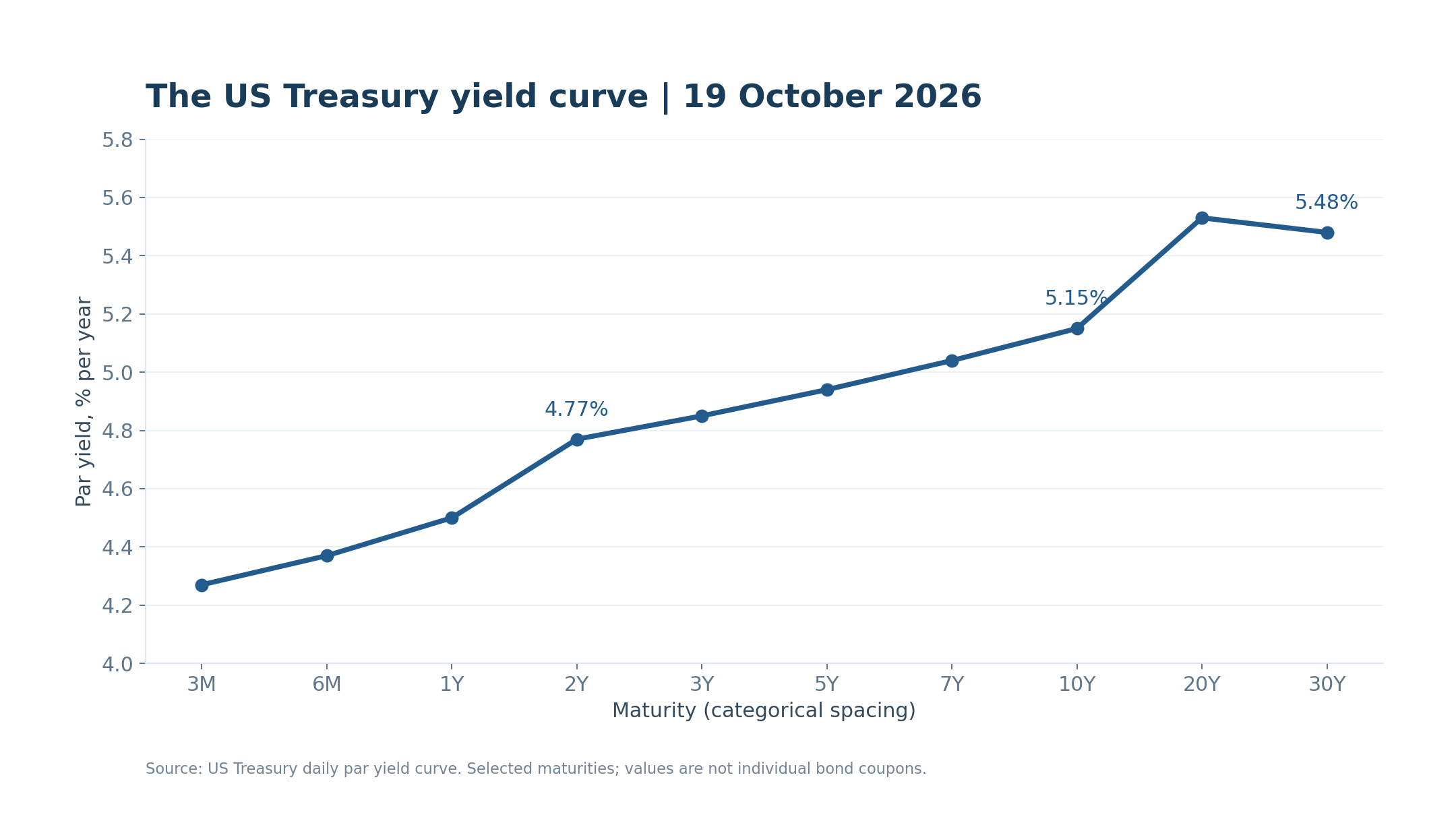
The yield curve plots yields against maturity. The two-year point is particularly sensitive to the expected policy path; the ten-year point combines that outlook with longer-term risks. The thirty-year point is useful for judging the price investors demand for committing capital far into the future. None is a pure measure of just one economic variable.

Curve terminology describes the route, not a recommendation. A bull steepening usually means yields decline with shorter maturities falling faster; a bear steepening means yields rise with longer maturities rising faster. An inverted curve means a shorter maturity yields more than a longer one. Its historical signalling value does not turn the slope into a precise timetable for recession or a certain date to buy risk assets.

On October 19, 2026, the Treasury reported two-year, ten-year and thirty-year par yields of 4.77%, 5.15% and 5.48%. The ten-year minus two-year spread was therefore +38 basis points. That upward slope says investors demanded more yield for longer lending. By itself, it does not prove that growth is healthy or that a recession is impossible.

Supply and demand deserve the same attention as macroeconomic forecasts. More long-dated issuance can require investors to absorb additional duration. Pension demand, foreign reserve management and central-bank holdings can work in the other direction. The effect depends on what was expected and on the willingness of buyers to hold the debt at prevailing prices. More issuance does not translate into an automatic, fixed increase in yields.

A curve can steepen because short yields fall on expected rate cuts, or because long yields rise on inflation and supply concerns. Those paths have very different implications. At auctions, compare demand, the auction yield with the pre-auction market, and subsequent trading; one weak auction is evidence to assess, not a standalone crash signal.

Term premium itself is not directly observable like the price of a traded bond. Analysts estimate it using models, surveys and assumptions about future short rates. Such estimates can help frame the debate, but a precise model number should not be mistaken for a separately measured market fact. The curve is observable; the decomposition explaining it is partly an analytical construction.

US Treasury daily par yields, 19 October 2026.View original ↗

A nominal yield is quoted in dollars without adjusting for future inflation. A real yield is linked to purchasing power. For a simple one-year illustration, a 5% nominal return with 3% inflation delivers about 1.94% real growth: 1.05 divided by 1.03, minus one. Subtracting inflation gives a useful approximation, but the exact relationship is multiplicative.

For an investor, the distinction concerns the spending power of future payments. A nominal Treasury promises a specified dollar principal, while a TIPS investment links principal to the relevant inflation index. Neither makes the investor immune to market-price changes before sale. A real yield can rise and the market price of an existing TIPS can fall even while its inflation adjustment increases the principal used for coupon calculations.

A hypothetical comparison illustrates the trade-off. If nominal bonds offer 5% and similar-horizon inflation-linked bonds offer around 2%, investors are comparing a fixed dollar return with an inflation-linked structure at a lower quoted real yield. Which performs better depends on realised inflation, purchase prices, cash-flow timing and other details. The approximate 3-percentage-point gap helps organise the comparison without settling the future outcome.

For market analysis, TIPS yields are more useful than subtracting the latest twelve-month CPI figure from a ten-year Treasury yield. The CPI release describes past inflation; both bond markets price future conditions. Comparing nominal Treasuries with similar-maturity TIPS gives an inflation-compensation measure commonly called breakeven inflation.

Breakeven inflation is not a clean forecast. It also reflects inflation risk compensation, liquidity differences and security-specific effects. On October 19, the published ten-year nominal and real par yields were 5.15% and 2.80%. Their simple difference was 2.35 percentage points—a useful rough indication of inflation compensation, not a matched-security breakeven calculation.

Expected inflation and inflation uncertainty are also different. Investors might retain the same central forecast while becoming less confident about it. They may then demand a larger premium for bearing inflation risk. This can move market inflation compensation even without an equivalent change in the most likely inflation outcome. Liquidity differences between markets can create an additional wedge during periods of stress.

Real yields are not a complete measure of monetary tightness either. A business borrows at its own financing rate, not necessarily at the TIPS yield. Consumers, governments and companies face different credit conditions and repayment schedules. Nevertheless, a change in long real yields provides a useful benchmark for how investors price an inflation-adjusted return on comparatively low-credit-risk dollar assets.

This distinction changes the interpretation of a bond sell-off. If nominal yields rise mainly because real yields increase, the competitive return on inflation-protected dollar assets improves. If inflation compensation rises instead, the message is more about purchasing-power uncertainty. Both can raise nominal yields while producing different outcomes for gold and risk assets.

For cross-asset analysis, separate the questions in order. Did the nominal yield change? How much did the real-yield benchmark change? Did the approximate inflation-compensation gap widen or narrow? Then compare the answer with the dollar, funding and the asset’s own news. This avoids explaining every rise in yields as “inflation” or every decline as “easier money” when the underlying components tell a more specific story.

Gold pays no contractual coupon. Higher real yields increase the income forgone by holding it instead of an inflation-protected government bond. A stronger dollar can add pressure on the dollar gold price. Falling real yields often ease those headwinds, making the real-yield trend a useful part of a precious-metals dashboard.

Opportunity cost works through choice rather than through a compulsory flow of money. An investor deciding between gold and a Treasury compares expected protection, income, liquidity and risk. Higher real bond income can make gold less attractive at the margin, but it does not force existing holders to sell. Their reasons for owning it may involve reserve diversification, portfolio insurance or a longer horizon than the next interest-rate cycle.

Yet gold is also held as reserve diversification and insurance against financial or geopolitical uncertainty. Those motives can outweigh the income comparison. Gold rising alongside yields is therefore possible: investors may be paying for protection even as the opportunity cost increases. The relationship is conditional, and a chart of yields alone cannot establish what is driving gold on a particular day.

A hypothetical disinflation scenario is relatively straightforward: inflation expectations remain anchored, real yields ease and the dollar weakens without a severe growth shock. That combination removes several obstacles for gold. Silver may also benefit if industrial demand remains resilient. The assessment becomes less straightforward when real yields fall because investors expect a deep contraction and simultaneously seek cash or reduce leverage.

During acute funding stress, even a defensive asset can be sold to meet obligations elsewhere. A brief gold decline during a broad sell-off therefore does not establish that its longer-term defensive role has disappeared. Timing matters: the initial need for liquidity and the subsequent response to recession risk can produce different price behaviour. A portfolio needs enough liquidity to avoid being forced into that initial sale.

Silver shares some monetary characteristics with gold but also has substantial industrial demand. A growth scare can therefore support defensive demand for gold while hurting silver through weaker expectations for manufacturing. Mining equities add another layer: energy costs, operating performance, financing and political exposure can dominate the metal-price effect.

The difference between bullion and mining shares is equally important. A producer receives revenue from selling metal but also pays wages, power bills, development costs and taxes. A higher gold price does not guarantee wider margins if operating costs rise faster. Royalty and streaming models have different exposures, while every company still requires an assessment of valuation, counterparties and capital allocation.

The practical question is whether the yield move is changing real financing conditions or revealing a demand for protection. If real yields rise but gold holds firm, investigate flows and risk demand before declaring the relationship broken. If yields fall because the economy is weakening, avoid assuming that silver or miners must benefit as much as gold.

For a mixed metals portfolio, a useful scenario exercise is to ask which holding is intended to provide insurance and which depends on industrial growth or operating leverage. Gold, silver and miners may all appear under a precious-metals heading, yet their response to a yield decline can differ markedly. Position sizing should reflect those differences instead of relying on one broad correlation with Treasuries.

Stocks: discount rates and earnings

For equities, Treasury yields help anchor the discount rate applied to future cash flows. In a simplified example, $100 received in ten years is worth about $61.39 at a 5% discount rate and $55.84 at 6%. That 9% reduction occurs without changing the future payment. Actual equity discount rates also include a risk premium, which can move independently.

Discounting alone does not value a whole business. Investors also estimate future sales, margins, investment needs and the probability that those forecasts are achieved. A growing company may justify a higher valuation despite a rising Treasury benchmark if its cash-flow outlook improves enough. A company with disappointing earnings can fall even when the risk-free component of its discount rate becomes more favourable.

Companies whose investment case rests on distant profits can be particularly sensitive. Borrowers, property companies and capital-intensive businesses also face refinancing costs. But stronger economic growth may lift earnings enough to offset higher yields. Conversely, recession fears can reduce yields while falling earnings expectations and a rising equity risk premium push share prices lower.

Credit spreads make the apparent contradiction especially clear. In a hypothetical growth scare, the Treasury benchmark falls by 0.30 percentage points but a weaker company’s credit spread widens by 0.80 points. Its indicative borrowing cost increases by 0.50 points overall. Falling government yields have not rescued the company’s financing outlook. The same logic helps explain why financially strong and highly leveraged businesses can diverge.

Sector labels are not sufficient. Technology businesses with distant expected profits can be rate-sensitive, but established profitable firms and speculative companies are not interchangeable. Banks face their own mix of asset yields, deposit costs and credit losses. Property and infrastructure businesses depend on refinancing schedules and cash-flow resilience. The question is where the changed cost of capital reaches the individual business. For both segments, the useful test is whether easier financial conditions are being confirmed by economic results rather than only a temporary improvement in investor sentiment.

Crypto: funding and demand

Bitcoin and most cryptoassets do not have bond-like promised cash flows, so the equity valuation formula cannot simply be applied to them. The transmission runs through the attractiveness of dollar income, access to funding, leverage and appetite for risk. Easier conditions can support crypto, while liquidations or a stronger dollar can amplify pressure.

In crypto, leverage can make this transmission faster. A leveraged trader facing tighter funding or losses may close positions regardless of a token’s long-term narrative. Liquidations can then push prices further and trigger additional selling. Conversely, a modest improvement in funding can produce a sharp rebound after crowded bearish positioning. Such a rebound does not by itself prove a lasting change in demand or network fundamentals.

Stablecoin yields and tokenised Treasury products also make the income alternative more visible to crypto investors, but these products add issuer, custody, legal or technical risks of their own. They should not automatically be treated as identical to directly held government debt. Compare the asset actually owned, the claim it provides and the route to redemption before comparing its displayed yield with a Treasury benchmark.

Crypto also has its own drivers: fund flows, regulation, token supply, network activity and market positioning. A decline in Treasury yields is useful context, not a buy signal for Bitcoin or every altcoin. A stronger setup combines easing real yields and stable funding with evidence that demand for the asset itself is improving.

For portfolio decisions, combine the macro backdrop with evidence at the asset level. In equities this means earnings quality and balance-sheet capacity; in crypto it means flows, leverage, token supply and economic use. A yield signal can justify more patience or a smaller position. It cannot substitute for deciding what the investment is worth and what evidence would invalidate the thesis.

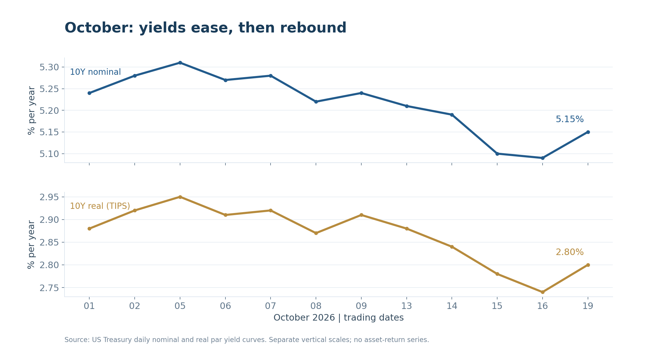
As of October 20, the Treasury’s October 19 observations show a partial retreat from early-month yields rather than a complete reversal. Between October 1 and October 16, the ten-year nominal yield fell from 5.24% to 5.09%, while the ten-year real yield fell from 2.88% to 2.74%. On October 19 they rebounded to 5.15% and 2.80%, respectively.

The earlier decline and the later rebound should be evaluated at two horizons. Relative to October 1, the ten-year nominal and real benchmarks were still lower on October 19. Relative to October 16, both were higher. A commentator can therefore describe either relief or renewed pressure and be arithmetically correct. The investment implication depends on whether the discussion concerns the monthly trend or the latest change.

The rebound was six basis points in both series. The simple nominal–real gap consequently remained 2.35 percentage points from October 16 to October 19. This arithmetic is consistent with the latest rise being concentrated in the real-yield component of these published curves. It does not identify which news item, trade or investor caused the move.

A six-basis-point move is small compared with a full percentage point, but its effect is not identical across instruments. For an illustrative bond with modified duration eight, a parallel six-basis-point rise implies roughly a 0.48% price decline before income and convexity. The same yield move does not imply a 0.48% fall in stocks, gold or Bitcoin: those assets do not share that bond’s contractual cash-flow sensitivity.

The 2.35-percentage-point nominal–real gap also needs proportion. Its stability over these two observations suggests little change in this rough inflation-compensation comparison, but it does not establish that inflation uncertainty was unchanged in every market. Nor does it reveal whether investor positioning amplified the move. This is a useful decomposition of the observed benchmarks, not a complete explanation of market behaviour.

For gold, that rebound restored some opportunity-cost pressure. For growth equities and crypto, it made the interest-rate backdrop less supportive than it had looked on October 16. These are implications of the framework, not claims that each asset actually moved by a particular amount or that Treasury yields were its sole driver.

Three subsequent paths would carry different messages. Continued easing in real yields with resilient earnings would improve the valuation backdrop. A renewed rise in real yields without stronger earnings would make the hurdle more demanding. A sharp decline in Treasury yields alongside widening credit spreads would point towards a growth or funding problem, where defensive demand and pressure on risk assets could coexist.

The useful next test is persistence. A sustained decline in real yields alongside stable growth expectations would be more constructive than a single favourable session. A rise in long yields without better earnings expectations would be harder for valuations. If stocks fall while yields ease, check credit spreads and earnings revisions before treating the divergence as irrational.

The disciplined response is to update the scenario rather than announce a turning point. For an existing position, ask whether the latest move changes the financing assumptions behind it. For a new position, ask whether the expected return still compensates for uncertainty if yields stay elevated longer. This turns the October observations into a decision framework without inventing a precise Treasury-driven price target for another asset.

Ten-year nominal and real par yields, October 2026. Separate vertical scales.View original ↗

Start with the two-year and ten-year yields, the ten-year TIPS real yield and the ten-year minus two-year spread. Compare changes over a week and a month as well as the latest session. This keeps a small daily reversal in proportion and helps distinguish a policy repricing from a broader change in long-term financing conditions.

A repeatable routine needs a time horizon. For a trade lasting several weeks, the path of yields, earnings expectations and positioning can matter more than a very distant equilibrium estimate. For capital intended for many years, valuation, reinvestment and the ability to tolerate drawdowns become more important. Decide which question the dashboard is meant to answer before interpreting every daily movement as relevant.

Then ask what changed. Was inflation unexpectedly strong? Did growth or employment weaken? Was there heavy issuance or an important auction? Compare the dollar, corporate credit spreads and equity market breadth. Falling yields with calm credit markets suggests a different environment from falling yields with widening spreads and forced selling.

Write down a small scenario set before acting. In a constructive case, inflation moderates without a serious earnings contraction and real yields ease. In an adverse valuation case, real yields rise while business prospects fail to improve. In a recession case, government yields decline but credit spreads widen and earnings expectations deteriorate. Identify which holdings are most vulnerable in each case and what evidence would distinguish them.

A simple decision note can contain the observed yield change, the most plausible explanation, a competing explanation and the market evidence still needed. For example, “real yields eased, but credit spreads widened” should prompt a different conclusion from “real yields eased and corporate funding remained calm”. Explicitly recording the competing interpretation reduces the temptation to select only the evidence that supports an existing position.

Finally, connect the evidence to the asset. For gold, assess real yields and defensive demand; for silver, add industrial conditions. For equities, examine earnings and refinancing needs. For crypto, add flows, leverage and token-specific developments. Treat these as interacting influences rather than independent checkboxes that guarantee a forecast.

Position size then connects interpretation to risk. Investors do not need certainty about the next move to avoid a concentration that only works under one favourable scenario. Cash needs, refinancing exposure and the combined sensitivity of several holdings deserve attention together. Owning gold, growth stocks and crypto does not necessarily create three independent risks if all positions rely on the same easing in real yields.

The Treasury market is valuable because it reveals how investors price time, inflation and uncertainty in dollars. It can improve position sizing, patience and the interpretation of market news. Its strongest contribution is a better question—why is the price of money changing?—followed by an assessment of whether the asset’s fundamentals support the trade.

Finally, compare the outcome with the original thesis rather than with a single forecast headline. Was the expected economic mechanism correct? Did company or token fundamentals offset it? Did excessive leverage turn a manageable view into an unmanageable position? These questions make Treasury analysis more useful over time. The objective is a better decision process and a portfolio that can survive being early or wrong—not a claim that one macro indicator can predict every price.